Project: Traffic Sign Classification
추천 : Paper with code
Implement and train a convolutional neural network to classify traffic signs. Use validation sets, pooling, and dropout to choose a network architecture and improve performance.
Human performance, 98.84%
Sujay Babruwad의 해결 방안
1. 전처리
- Gray scale 이미지로 변경 : 도로 표지판들이 비슷한 색상 패턴을 가지고 있으므로
빨강 & 파란색이 영향을 미치지 않나??
- 추가 이미지 생성 : Images will mostly appear skewed or ‘perspective-transformed’ in real life applications
- Rotation, Skewing and translation are applied to these images
2. 본처리
텐서플로우를 사용하여 5계층의 레이어 생성
Layer 1: Convolution of 5x5 kernel, 1 stride and 16 feature maps
- Activation: ReLU
- Pooling: 2x2 kernel and 2 stride
Layer 2: Convolution of 5x5 kernel, 1 stride and 32 feature maps
- Activation: ReLU
- Pooling: 2x2 kernel and 2 stride
Layer 3: Fully connected layer with 516 units
- Activation: ReLU with dropout of 25%
Layer 4: Fully connected layer with 360 units
- Activation: ReLU with dropout of 25%
Layer 5: Fully connected layer with 43 units for network output
Activation Softmax
Adam optimizer with learning rate of 0.001
- weights initialized with mean of 0 and standard deviation of 0.1 are chosen
- batch size 256 and 100 epochs
3. 후처리
The validation accuracy attained 98.2% on the validation set and the test accuracy was about 94.7%
4. 결과
hengcherkeng의 해결 방안
[Jupyter]/001/Traffic_Sign_Classifier.ipynb), [GitHub], [Report]
0. 개요
1. 전처리
I use convolution net to do data pre-processing.
- It consists of 3x3 and 1x1 filters and trainable parametric ReLU[1]
# the inference part (without loss)
def DenseNet_3( input_shape=(1,1,1), output_shape = (1)):
    H, W, C   = input_shape
    num_class = output_shape
    input     = tf.placeholder(shape=[None, H, W, C],
                           dtype=tf.float32, name='input')
    # color preprocessing using conv net:
    # we use learnable prelu (different from paper) and 3x3 onv
    with tf.variable_scope('preprocess') as scope:
        input = bn(input, name='b1')
        input = conv2d(input, num_kernels=8, kernel_size=(3, 3),
                  stride=[1, 1, 1, 1], padding='SAME',
                  has_bias=True, name='c1')
        input = prelu(input, name='r1')
        input = conv2d(input, num_kernels=8, kernel_size=(1, 1),
                  stride=[1, 1, 1, 1], padding='SAME',
                  has_bias=True, name='c2')
        input = prelu(input, name='r2')
    with tf.variable_scope('block1') as scope:
        block1 = conv2d_bn_relu(input, num_kernels=32,
                    kernel_size=(5, 5), stride=[1, 1, 1, 1],
                    padding='SAME')
        block1 = maxpool(block1, kernel_size=(2,2),
                    stride=[1, 2, 2, 1], padding='SAME')
...
For data augmentation
- I generate new data during the learning epoch.
- I have to be careful that the data cannot change too much for each epoch or else I will see “jumps in the loss”.
- To do this I kept some percentage of the data consistent (e.g. random 20%) and use it for E epoch before generating new data.
loop for R runs
    generate augmented data.
    train data = 20% of original data + 80% augmented data
    loop for E epoch
       perform sgd on train data for a few epoch until,
       data is fairly exhausted.
#note: total number of epoch used in training = R*E
Here is the secret sauce! Illumination augmentation makes the difference. The code for illumination augmentation is:
#brightness, contrast, saturation-------------
#from mxnet code, see: https://github.com/dmlc/mxnet/blob/master/python/mxnet/image.py
if 1:  #brightness
    alpha = 1.0 + illumin_limit*random.uniform(-1, 1)
    perturb *= alpha
    perturb = np.clip(perturb,0.,255.)
    pass

if 1:  #contrast
    coef = np.array([[[0.299, 0.587, 0.114]]]) #rgb to gray (YCbCr) :  Y = 0.299R + 0.587G + 0.114B

    alpha = 1.0 + illumin_limit*random.uniform(-1, 1)
    gray = perturb * coef
    gray = (3.0 * (1.0 - alpha) / gray.size) * np.sum(gray)
    perturb *= alpha
    perturb += gray
    perturb = np.clip(perturb,0.,255.)
    pass

if 1:  #saturation
    coef = np.array([[[0.299, 0.587, 0.114]]]) #rgb to gray (YCbCr) :  Y = 0.299R + 0.587G + 0.114B

    alpha = 1.0 + illumin_limit*random.uniform(-1, 1)
    gray = perturb * coef
    gray = np.sum(gray, axis=2, keepdims=True)
    gray *= (1.0 - alpha)
    perturb *= alpha
    perturb += gray
    perturb = np.clip(perturb,0.,255.)
    pass
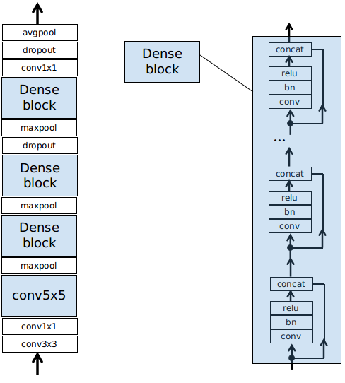
2. 본처리
For network design,
- I try to use the least number of conv layers.
- I use batch normalization and some dropout.
- I choose to use Dense block because the concatenation basically connects the lower layer input all other layers at the top. This is a kind of “shortcut” and activation of different scales get to be combined.
Here is the MAC1 computation

3. 후처리
4. 결과 / Insight
데이터의 양이 적다 : 이 경우 Overfit된어 Train에러는 작지만, Test에러는 크게 나타난다.
- 해결책 : data augmentation, regularization
Data is too complex : 이 경우 Train에러는 크다.
- 해결책 : design a more complex and usually deeper network
- 그러나 Deep network는 Train하기 쉽지 않다. 딥네트워크는 Inception block, residual block and dense block등으로 구성되고, batch normalization도 해야 한다.
- 또는 You can make the data less complex(representation, 전처리 이용). Break the problem into smaller and simpler ones(cascaded, hierarchical networks이용)
Jessica Yung의 해결 방안
[Jupyter]/001/Traffic_Sign_Classifier.ipynb), [GitHub], [Report]
이미지 전처리 부분만 다룸
0. 개요
- Normalised the data
- Did not use convolutions
이미지 전처리 부분만 다룸
1. 전처리
Normalisation: 모든 값을 0~1사이의 값으려 변환
- 단점 : 데이터에 아웃라이어가 있으며 제대로 동작 안함. 대부분의 데이터들은 아웃라이어가 있음
Standardisation : transforms your data to have a mean (average) of zero and a variance of one
- 단점 : Your new data usually aren’t bounded, unlike normalisation.
Normalise 해야 하는 이유 : The same range of values for each of the inputs to the neural network can
guarantee stable convergence of weights and biases
# Standardise input (images still in colour)
X_train_std = (X_train - X_train.mean()) / np.std(X_train)
X_test_std = (X_test - X_test.mean()) /np.std(X_test)
# Normalise input (images still in colour)
X_train_norm = (X_train - X_train.mean()) / (np.max(X_train) - np.min(X_train))
X_test_norm = (X_test - X_test.mean()) / (np.max(X_test) - np.min(X_test))

- Sometimes standardising images can transform them from readable to humanly unreadable:
- Normalising images brings out features we wouldn’t have been able to see otherwise.
Waleed Abdulla의 해결 방안
기타 참고 자료
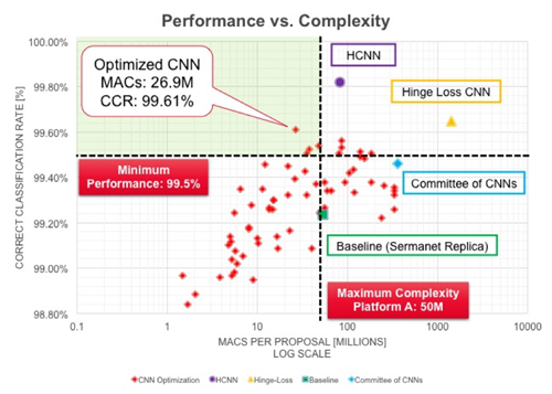
Spatial transformer network, 99.61%, [Link1], [Link2]
- For data pre-processing, they use spatial transformer network to align the input data.
Alex Staravoitau solution, 99.33%, [Link
- For data pre-processing, histogram equalization is used.
- For network design, there is some skipping connections. Activation of different scales are concatenated and feed to the last fully connect layer.
Vivek Yadav solution, 99.10%, [Linke1], [Link2]
- For data augmentation, brightness perturbation is used in additional to geometric perturbation.
- For network design, there is some skipping connections like Alex’s solution above.
Industrial performance (e.g. Cadence) , 99.82%, [Link1], [Link2], [Link3]
- For network design, hierarchical network is used.

1. multiply–accumulate operation counts ↩
[1] “Systematic evaluation of CNN advances on the ImageNet”- Dmytro Mishkin, Nikolay Sergievskiy, Jiri Matas, ARXIV 2016.