Project: Behavioral Cloning Architect and train a deep neural network to drive a car in a simulator. Collect your own training data and use it to clone your own driving behavior on a test track.
Jeremy Shannon의 해결 방안
0. 개요
- 핸들 각도 분포에 따른 성능 평가
1. 전처리
- Udacity에서 제공한 Train 이미지는 전처리 작업 필요 : cropping, resizing, blur, and a change of color space)
- Then I introduced some “jitter” (random brightness adjustments, artificial shadows, and horizon shifts) to sort of keep the model on its toes, so to speak
- Udacity에서 테스트는 직선 길이가 많다. 그래서 운전대도 대부분 0각도에 많이 치우쳐져 있다.
- 이렇게 되면 급커드 도로에서는 제대로 대처 하지 못한다.
- 중앙에 치운친 값들을 제거 하여 완만하게 변경
- 추가 적인 전처리 과정들
- More aggressive cropping (inspired by David Ventimiglia’s post)
- Cleaning the dataset one image at a time (inspired by David Brailovsky’s post)
2. 본처리
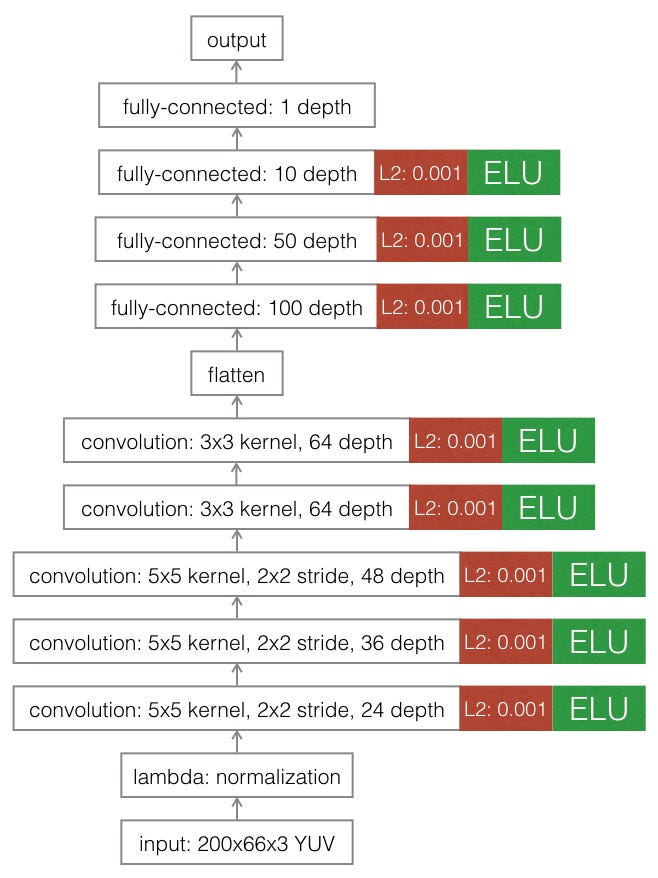
- Further model adjustments (L2 regularization, ELU activations, adjusting optimizer learning rate, etc.)
- Model checkpoints (something of a buy-one-get-X-free each time the training process runs)
3. 후처리
4. 결론
- 성능은 데이터에 달려 있음.
- 모델 아키텍쳐를 바꾸는것은 큰 효과가 없음
- 급 커브에 대응 하려면 그러한 데이터도 있어야 함.
좀더 자세한 기술은 [여기]참고
Arnaldo Gunzi의 해결 방안
0. 개요
- Inputs: Recorded images and steering angles(8036*3 : 중앙, 오른쪽, 왼쪽 카메라), throttle, brake.
- The steering angle is normalized from -1 to 1, corresponding in the car to -25 to 25 degrees.
- Outputs: Predicted steering angles
- What to do: Design a neural network that successfully and safely performs the circuit by himself
잘 되지 않음. 무엇이 영향을 미치는지 고찰 필요 : 구름, 강, 차선, 도로 색상, 차선이 없으면?
1. 전처리
1.1 Image augmentation
A. Center and lateral images
- 좌/우측의 카메라 정보를 사용할수 없을까?
- I added a correction angle of 0.10 to the left image, and -0.10 to the right one. The idea is to centre the car, avoid the borders.
B. Flip images
- 일부 이미지를 좌우 대칭 & 운전대 각도 변경
- we can neutralize some tendency of the human driver that drove a bit more to the left or to the right of the lane.
if np.random.uniform()>0.5:
  X_in[i,:,:,:] = cv2.flip(X_in[i,:,:,:],1)
  Y_in[i] = -p[i] #Flipped images
C. Random lateral perturbation
- The idea is to move to image a randomly a bit to the left or the right,
- and add a proportional compensation in the angle value.
D. Resize

- 성능상의 문제로 이미지크기가 작으면 좋다.
- stride of the convolutional layers도 줄였다.
신기한 결과 : When the image is smaller, the zig zag of the car is greater. Surely because there are fewer details in the image.
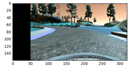
E. Crop
하늘과 나무들을 삭제
crop_img = imgRGB[40:160,10:310,:] #Throwing away to superior portion of the image and 10 pixels from each side of the original
image = (160, 320)
F. Grayscale, YUV, HSV
I tried grayscale, full color, the Y channel of YUV, S channel of HSV
- All of this because my model wasn’t able to avoid the dirty exit after the bridge, where there is not a clear lane mark in the road.
 imgOut = cvtColor(img, cv2.COLOR_BGR2YUV)
 imgOut = cvtColor(img, cv2.COLOR_BGR2HSV)
G. Normalization
뉴럴 네트워크는 작은 수에 잘 동작 하기에 Normalization 실시
- sigmoid activation has range (0, 1), tanh has range (-1,1).
Images have 3 RGB channels with value 0 to 255.
- The normalized array has range from -1 to 1 :
X_norm = X_in/127.5–1
2. 본처리
뉴럴 네트워크의 종류는 많기 때문에 일단 시작으로 NVIDIA 모델을 적용 하였다[1].
3. 후처리
4. 결론
전처리에 대한 대부분을 커버 하고 있음
James Jackson의 해결 방안
0. 개요
1. 전처리
Data Augmentation
- Smoothing steering angles & normalizing steering angles based on throttle/speed, are both investigated
- A constant 0.25 (6.25 deg.) is added to left camera image steering angles, and substracted from right camera image steering angles
- This forces aggressive right turns when drifting to the left of the lane, and vice-versa.
- Variable steering adjustment based on the current steering angle is an area for future investigation.
- All images (left, center, right) are flipped to provide additional data & balance the dataset
- 불필요한 상하단 이미지 제거
- 학습 시간 단축을 위해 resized to 64x64 pixels
더 자세한 augmentation은 Vivek Yadav 참고
2. 본처리
2.1 The Model
comma.ai의 학습모델을 기본으로한 Tensorflow/Keras 이용
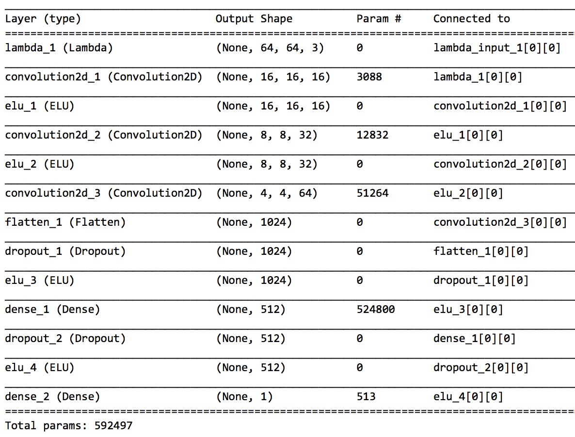
- The input layer takes a 64x64x3 (RGB) image and normalizes the values between -1 and 1 via a lambda funtion.
- There are 3 convolutional layers
- using 16 filters of size 8x8
- 32 filters of size 5x5
- finally 64 filters of size 5x5.
- The convolutional layers are separated by activation layers, specificially Exponential Linear Units (ELUs).
- DropOut
- dropout (0.2) is applied before switching to the first fully connected layer.
- A second dropout (0.5) is applied before the final fully connected layer of 513 parameters.
- The dropouts create a robust network that is more resilient to overfitting.
- The model uses 592,497 parameters in total. 0.0194 after the 8th
2.2 Training
- Adam optimizer(learning rate of 0.001 )
- Training is run for 8 epochs
- Mean Squared Error (MSE) : 1st epoch is 0.0327 -->
3. 후처리
4. 결론
Alena Kastsiukavets의 해결 방안
0. 개요
Transfer Learning with Feature Extraction 기법 적용
- this approach is chosen when your NN is similar to base network
- We have a pre-trained neural network from ImageNet Competition
- ImageNet모델은 Object탐지에 좋은 성능을 보이고 있고, 차선도 Object의 하나이다.
Transfer Learning기법의 장점
- 많은 데이터가 불필요하다. 따라서 유다시티 ~8.000로도 충분하다.
- Thanks to frozen weights and small amount of images (I use ~400 images) I have significantly reduced training time and was able to play a lot with my car and analyze its behavior.
- I had a small hope that pre-trained NN would help me to generalize to track 2 without heavy data-augmentation.
- Unfortunately, I had to add brightness augmentation to generalize to track2.
1. 전처리
- cropping to remove unnecessary information from the image
- applied random brightness for every image from tests set
2. 본처리
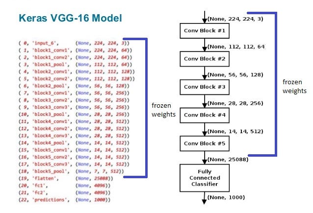
- Feature extraction를 위한 모델로 VGG16 이용
- It has good performance and at the same time quite simple.
- Moreover it has something in common with popular NVidia and comma.ai models.
- VGG16을 이용하기 위해서는 최소 48x48크기의 Color이미지를 사용해함
3. 후처리
4. 결론
There is a list of techniques I found useful for this project:
- 항상 코드를 재 확인해라. 사소한 실수들이 내재되어 있을수 있다. 저자는 초기에 실수로 검은 사진만 학습에 사용하였다.
- 여러 기술들을 한번에 적용해보고 싶겠지만, 하나씩 적용해 가면서 살펴 보는게 중요하다. And tuning became easy and predictable!
- 데이터의 균형을 이루어라 Balance your data! It is the key point.
- When your model is good, validation loss is a good indicator of better model.
- Before this it is good to use callbacks and save your model after each iteration.
- They allow you to analyze your model behavior! [참고]
Denise R. James의 해결 방안
0. 개요
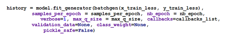
- Keras `modle.fit_generator()를 효율적으로 이용
코드 설명은 본문 [참고]
1. 전처리
- 상하단 이미지 제거
2. 본처리

2.1 First Conv. Layer - Conv1
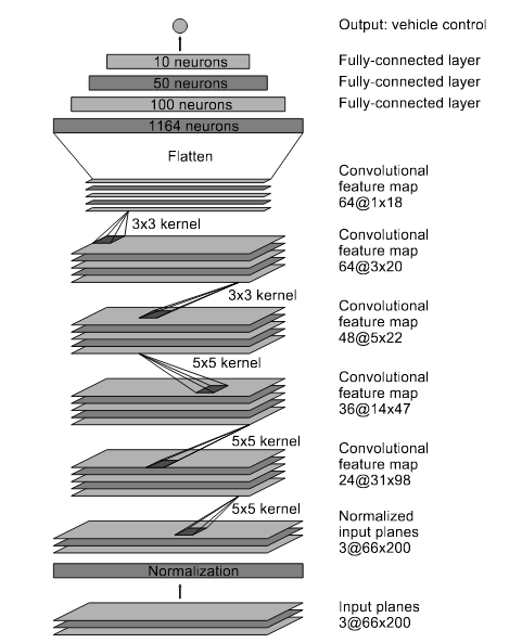
For the input planes with a shape of 66x208x3, (HxWxD) conv1 has 24 filters of shape 5x5x3 (HxWxD) A stride of 2 for both the height and width (S) Same padding of size 1 (P) The formula for calculating the new output height or width of conv1 layer is: new_height = (input_height — filter_height + 2 P)/S + 1 new_width = (input_width — filter_width + 2 P)/S + 1 new_height = (66–5 +21)/2 +1 = 33 new_width = (208–5+21)/2 + 1 = 104 Output shape of conv1 layer is (33, 104, 24)
2.2 Second Conv. Layer - Conv2
For the input planes with a shape of 33x104x24, (HxWxD) conv2 has 36 filters of shape 5x5x24 (HxWxD) A stride of 2 for both the height and width (S) Same padding of size 2 (P) The formula for calculating the new output height or width of conv1 layer is: new_height = (input_height — filter_height + 2 P)/S + 1 new_width = (input_width — filter_width + 2 P)/S + 1 new_height = (33–5 +22)/2 +1 = 17 new_width = (104–5+22)/2 + 1 = 52 Output shape of conv1 layer is (17, 52, 36) Parameters = (5 x 5 x 24 + 1 ) *36 = 21636
2.3 Third Conv. Layer - Conv3
이후 레이어 설명은 본문 [참고]
3. 후처리
Andrew Wilkie의 해결 방안
0. 개요
 Keras를 이용하여 구현
- truncated highly logged angles to reduce bias,
- shifted left and right front facing driving images with corresponding steering angles adjustments to generate Recovery training examples, instead of manually recording them,
- cropped the camera images to the road and low horizon to help the model focus it’s learning on the important features of the image,
- randomly applied shadows to the training dataset as Test Track 2 is dark, and
- randomly mirrored the images and their corresponding steering angles to reduce the left-steering bias in the training dataset.
1. 전처리
Vivek Yadav’s의 방식 적용
- An augmentation based deep neural network approach to learn human driving behavior
2. 본처리
Nvidia model 모델 사용
3. 후처리
4. 결과
1 “End to End Learning for Self-Driving Cars”- Mariusz Bojarski, ARXIV 2016.
1. Smoothing steering angles by SciPy Butterworth filter ↩