Project: Vehicle Tracking Track vehicles in camera images using image classifiers such as SVMs, decision trees, HOG, and DNNs. Apply filters to fuse position data.
Milutin N. Nikolic의 해결 방안
0. 개요
The goals/steps of this project are the following:
- Extract the features used for classification
- Build and train the classifier
- Slide the window and identify car on an image
- Filter out the false positives
- Calculate the distance
- Run the pipeline on the video
1. 전처리
2. 본처리
차량과 차량이 아닌것 분류 필요
- To build a classifier, first, the features have to be identified.
- The features that are going to be used is a
mixture of histograms,full images, andHOG-s.
2.1 Extracting features
A. Color space
- Color space is related to the representation of images in the sense of color encodings.
- 각각의 목적에 맞는 Color space가 있음, 분류 문제에 좋은 Color space가 정해져 있는건 아니므로 하나씩 시도 해보면서 찾아야 함
[저자의 접근 방법]
What I have done, is that I have built the classifier, based on HOG, color histograms, and full image and then changed the color space until I got the best classification result on a test set.

결론 : LUV color space works the best
B. Subsampled and normalized image as a feature
 첫번째 Feature : subsampled image
- Subsampled : 20x20로
- Gamma-normalised : 그림자 영향을 적게 받음??
- It was stated that taking a square root of the image
normalizes itand getsuniform brightnessthus reducing the effect of shadows
- It was stated that taking a square root of the image
Subsample? 이미지 중에 필요한 부분만 잘라 내는 것인가?
C. Histogram of colors
두번째 Feature : color histograms.
- A number of bins in a histogram is selected based on the testing accuracy and
128 binsproduce the best result.
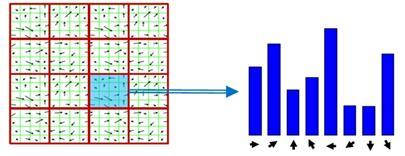
D. HOG
세번째 Feature : histogram of oriented gradients(HOG)
- The image on which the HOG is calculated is of size
64x64. - The number of pixels per cell is
8 - The number of cells per block is
1 - The number of orientations is
12
The HOG is calculated on all three channels of a normalized image
참고 : 매칭 방법과 HOG
Feature Description의 종류[1]
- 템플릿 매칭은 원래 영상의 기하학적 정보를 그대로 유지하며 매칭할 수 있지만 대상의 형태나 위치가 조금만 바뀌어도 매칭이 잘 안되는 문제가 있다.
- 히스토그램 매칭은 대상의 형태가 변해도 매칭을 할 수 있지만 대상의 기하학적 정보를 잃어버리고 단지 분포(구성비) 정보만을 기억하기 때문에 잘못된 대상과 매칭이 되는 문제가 있다.
- HOG는 중단 단계 매칭 방법
- 블록 단위로 기하학적인 정보를 유지하고, 각 블록 내부에서는 히스토그램을 사용하여 분포(구성비) 정보를 가지고 있는다.
- 이러한 특징때문에 지역적(local)인 변화에 대해 robust한 특성이 있다. 한글 설명
- HOG는 Image Detection(=물체를 탐지하기 위해 사용되는 Feature Descriptior)
- HOG는 방향을 Histogram의 Bin으로 정의
- 대상 영역을 일정 크기의 셀로 분활 - 각 셀마다 Edge의 방향에 대한 Histogram 생성
- ex: 어떤 위치에서 변화가 a만큼이고 방향이 b라면 b에 해당하는 bin에 a의 값만큼 더한 것
- 장점 : HOG는 edge의 방향정보를 이용하기 때문에 기본적으로 영상의 밝기 변화, 조명 변화 등에 덜 민감
- 활용 : 물체의 윤곽선 정보를 이용하는 사람, 자동차 등과 같이 내부 패턴이 복잡하지 않고 고유한 윤곽선 정보를 갖는 물체를 식별하는데 적합한 feature descriptor이다.
영문 설명
- The main idea around the HOG, is that histogram is calculated based on the orientations at each pixel calculated using some edge detector.
- Pixels that are on the edges contribute much more to the histogram than the edges that aren't.
- The image is divided in a number of cells and for each cell the orientations are binned.
- So the HOG basically shows the dominant orientation per cell.
2.2 Training the classifier
The classifier used is linear support vector classifier and trained with C=1e-4
- If the difference between the two accuracies is high the training is overfitting the data so the C was
lowered - When the test accuracy is low but same as training accuracy, the underfitting has occurred so the value of the C was
increased
3. 후처리
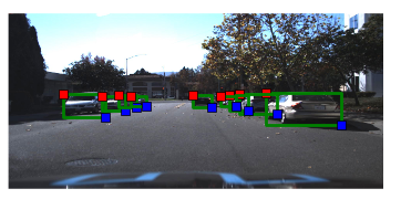
3.1 Calculating the heatmap and identifying cars
- Since there are multiple detections of the same car the windows had to be grouped somehow. - 히트맵(heatmap)사용
- Each pixel in the heatmap holds the number of windows with identified cars which contain that pixel.
- 값이 높을수록 차량의 부분일 가능성 높음
- The heatmap is thresholded with a threshold of 1, which removes any possible false car detections.
After that, the connected components get labeled and the bounding box is calculated. The resulting images are:

3.2 Removal of the road
- 목적 : 차량간의
거리를 측정 하기 위하여 - 이전 perspective transform[참고]을 통해서 maps the road surface to the image and enables us to measure distances확인
이부분을 이해 하기 위해서는 저자의 Advanced lane finding project를 이해하여야 함
추후 다시 확인
Vivek Yadav의 해결 방안(U-net)
0. 개요
U-net을 이용한 차량 탐지 [U-Net 홈페이지],
- U-net is a encoder-decoder type of network for pixel-wise predictions
- U-net is unique because in U-net, the receptive fields after convolution are concatenated with the receptive fields in up-convolving process
- This additional feature allows network to use original features in addition to features after up-convolution
- This results in overall better performance than a network that has access to only features after up-convolution.
1. 전처리
1.1 Data
- Udacity 데이터셋 이용 (차량, 트럭, 보행자)
- 차량 & 트럭을 하나의 분류로 합치고, 보행자 삭제
1.2 Data preparation and augmentation
A. stretching

- We first define 4 points near corners of the original image (shown in purple).
- We then stretch these points so these points become the new boundary points.
- We modify the bounding boxes accordingly
B. Translation
 We next apply translation transformation, to model the effect of car moving at different locations.
?? Translation에 대하여 다시 확인 필요
C. brightness augmentation
2. 본처리
2.1 Model
U-net 이용 : A scaled down version of a deep learning architecture
- 바이오 분야에서Cancer 탐지 하는데 주로 사용
- U-net is a encoder-decoder type network architecture for image
segmentation - the feature maps from convolution part in downsampling step are fed to the up-convolution part in up-sampling step
U-Net의 특징
- 학습 데이터양이 적을때도 좋은 성능을 보임 (less than 50 training samples)
- 입력 이미지 크기에 대한 요구 사항(=제약)이 없음
it does not have any fully connected layers, therefore has no restriction on the size of the input image. This feature allows us to extract features from images of different sizes, which is an attractive attribute for applying deep learning to high fidelity biomedical imaging data
- 입력: input to U-net is a resized 960X640 3-channel RGB image
- 출력: output is 960X640 1-channel mask of predictions.
- 활성함수: We wanted the predictions to reflect probability of a pixel being a vehicle or not, so we used an activation function of sigmoid on the last layer.
2.2 Training

- batch size of 1
- adam optimizer with a learning rate of 0.0001
- 10000 iterations
3. 후처리
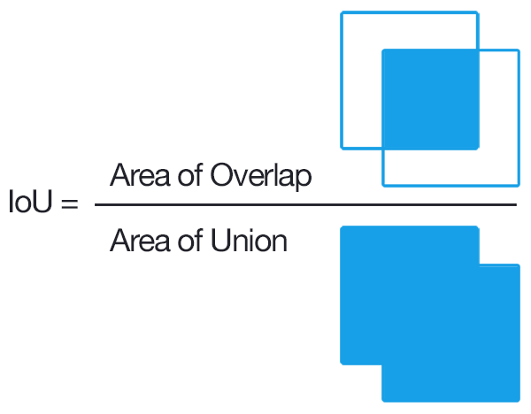
3.1 Objective:
We defined a custom objective function in keras to compute approximate Intersection over Union (IoU) between the network output and target mask.
- IoU is a popular metric of choice for tasks involving bounding boxes.
- The objective was to maximize IoU, as IoU always varies between 0 and 1, we simply chose to minimize the negative of IoU.
4. 결론
속도 : 20ms per image
Additional links:
Kaspar Sakmann의 해결 방안
0. 개요
- The ideal solution would run in real-time, i.e. >30FPS
- 2005년에 linear SVM와 HOG를 이용한 나의 방법은 measly 3FPS on an i7 CPU 였다.
- 이번에는 [YOLO][https://pjreddie.com/darknet/yolo/]를 이용하여 구현해 보려 한다. - 65FPS
1. 전처리
1.1 Feature Extraction
- spatial features: down sampled copy of the image patch to be checked itself (16x16 pixels)
- color histogram features: capture the statistical color information of each image patch.
- Cars often come in very saturated colors which is captured by this part of the feature vector.
- Histogram of oriented gradients (HOG) features: capture the gradient structure of each image channel and work well under different lighting conditions
- 3가지 방식(Each Image Channel)으로 특징을 추출 하였으므로 Scale을 조정할 필요가 있음
- It is therefore necessary to scale every feature to prevent one of the features being dominant merely due to its value range being at a different scale
- I therefore used the
Standard.Scalerfunction(=scikit패키지) tostandardize featuresby removing the mean and scaling to unit variance.
2. 본처리
Training a linear support vector machine
- 실시간 Object 탐지에서는 반드시 실시 해야 하는 부분
- 실시간 속도에 영향을 미치는 요소 : length of the feature vector & the algorithm
- A linear SVM offered the best compromise between speed and accuracy
- 다른 알고리즘 대비 : random forests (fast, but less accurate), nonlinear SVMs (rbf kernel, very slow)
YOLO에서는 사용하지 않아도 속도 좋은것 같음 (As no sliding windows are used the detection is extremely fast)
후처리
Sliding windows

차량 탐지를 위해 사용되는 필터 윈도우
- Shown below is a typical example of positive detections together with all ~150 windows that are used for detecting cars (= FALSE POSITIVE 존재)
- 해결법: I always kept track of the detected windows of the last 30 frames and more than 15 detections만 Positive로 간주
- 히트맵으로 표현 - 히트맵에 Thresodling하여 하나의 박스로 표현