Lidar Features

PCL/OpenNI tutorial 4: 3D object recognition (descriptors))

Feature 리스트

Feature요구 사항

1. It must be robust to transformations:
   • rigid transformations (the ones that do not change the distance between points) like translations and rotations must not affect the feature.
   • Even if we play with the cloud a bit beforehand, there should be no difference.
2. It must be robust to noise:
   • measurement errors that cause noise should not change the feature estimation much.
3. It must be resolution invariant:
   • if sampled with different density (like after performing downsampling), the result must be identical or similar.

Feature 후처리

계산후에는 식별자의 크기를 히스토그램들을 이용하여 줄여야 한다. After calculating the necessary values, an additional step is performed to reduce the descriptor size: the result is binned into an histogram.

• To do this, the value range of each variable that makes up the descriptor is divided into n subdivisions,
• and the number of occurrences in each one is counted

Using binned histograms provides the benefit or removing object detail, as the bin size decreases, which normalises the object features, allowing better classification against variations with an objects orientation, position or environmental lighting conditions. However, as the bin size decreases, detail is lost, and different objects begin to show the same characteristic's resulting in incorrect object classification.

대분류

• Global Descriptors
• Local Descriptors

1. Local descriptors

지역 기술자는 각 포인트들을 계산하다. Local descriptors are computed for individual points that we give as input.

단지, 주변 포인트들을 고려하여 local geometry가 어떤지를 기술한다. They have no notion of what an object is, they just describe how the local geometry is around that point.

대부분 사용자가 포인트의 어느 부분을 계산할지 선택 한다. Usually, it is your task to choose which points you want a descriptor to be computed for: the keypoints.

Most of the time, you can get away by just performing a downsampling and choosing all remaining points, but keypoint detectors are available, like the one used for NARF, or ISS.

지역 기술자는 물체 인식이나 Registration에 활용된다. Local descriptors are used for object recognition and registration.

1.1 PFH (Point Feature Histogram)

• PCL에서 제공하는 가장 중요한 기술자 이다. It is one of the most important descriptors offered by PCL and the basis of others such as FPFH.

• PFH은 주변 Normal 방향들의 차이점을 분석하여 기하학적 정보를 수집한다. The PFH tries to capture information of the geometry surrounding the point by analyzing the difference between the directions of the normals in the vicinity

  • 이때문에 부정확한 Normal을 기반으로 하면 기술자 질도 좋지 않다. (and because of this, an imprecise normal estimation may produce low-quality descriptors).

• 모든 포인들에 대하여 주변점들과 쌍을 생성한다. First, the algorithm pairs all points in the vicinity (not just the chosen keypoint with its neighbors, but also the neighbors with themselves).

• 그들의 Normal을 이용하여 fixed coordinate frame계산 Then, for each pair, a fixed coordinate frame is computed from their normals.

• 이 Frame을 이용하여 Normal간의 차별점을 계산 3각 변수로 정한다. With this frame, the difference between the normals can be encoded with 3 angular variables.

• These variables, together with the euclidean distance between the points, are saved, and then binned to an histogram when all pairs have been computed.

The final descriptor is the concatenation of the histograms of each variable (4 in total).

Point pairs established	Fixed coordinate frame and angular features computed for one of the pairs

1.2 FPFH (Fast Point Feature Histogram)

FPH는 계산 부하가 크다. For a cloud of n keypoints with k neighbors considered, it has a complexity of O(nk^2). FPFH의 시간 복잡도 : O(nk)

The FPFH considers only the direct connections between the current keypoint and its neighbors, removing additional links between neighbors. .

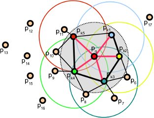Point pairs established

• To account for the loss of these extra connections, an additional step takes place after all histograms have been computed:
  • the SPFHs of a point's neighbors are "merged" with its own, weighted according to the distance.

• This has the effect of giving a point surface information of points as far away as 2 times the radius used.

• Finally, the 3 histograms (distance is not used) are concatenated to compose the final descriptor.

하영민, 손 및 팔의 자세 추정을 위한 다시점 뎁스 데이터의 3차원 정합, 2014

특정 점으로부터 일정 반경 내의 점들이 갖는 법선 백터들 간의 각도 관계를 표현하는 히스토 그램이다.

1. 임이의 두점에서의 법선 벡터를 기반으로 Darboux좌표계를 식 (1)과 같이 정의하고
2. 이를 기준으로 법선 벡터와 좌표계가 이루는 각도를 식 (2)와 같이 계산한다.

점군 데이터의 표면 법선 벡터를 기반으로

1. 질의점의 표면 법선 벡터와 목표점의 표면 법선 벡터를 기반으로 좌표계를 설정하고
2. 이 좌표계와 법선 벡터 사이의 관계를 수치화하여 특징 벡터를 구성하는 방법이다.

$$ uvw $$프레임 = $$ u $$축을 질의점의 표면법선 벡터 $$n_s$$로 설정 한다면, $$v$$축과 $$w$$축은 아래와 같다.

• 질의점 $$p_s$$의 표면 법선 벡터 = $$n_s$$
• 목표점 $$p_t$$의 표면 법선 벡터 = $$n_t$$

위와 같이 설정된 $uvw$프레임을 이용하여 표면법선벡터와의 관계를 수치화 할수 있다.

특징 벡터 $$ F= \< \alpha, \phi, \theta, d > $$ 계산식 (4차원)

• 점 사이 의 거리
• 법선 벡터와 좌표계의 축이 이루는 각도가 각 차원의 값

차이점

• 특히 FPFH 방식은 PFH와 달리 속도를 크게 개선한 방법으로 질의점 과 주변 점들 사이의 특징 벡터를 계산하고, 그것을 다시 활용하는 전략 을 이용한다.
• 이렇게 미리 저장한 특징 벡터를 활용하여 성능에는 큰 차이가 없게 하고, 속도를 크게 개선하였다.

1.3 RSD(Radius-Based Surface Descriptor)

• 타겟점과 이웃간의 반지름 관계 정보를 이용한다. The RSD encodes the radial relationship of the point and its neighborhood.

• For every pair of the keypoint with a neighbor, the algorithm computes

  • the distance between them, and
  • the difference between their normals.

• Then, by assuming that both points lie on the surface of a sphere, said sphere is found by fitting not only the points, but also the normals (otherwise, there would be infinite possible spheres).

• Finally, from all the point-neighbor spheres, only the ones with the maximum and minimum radii are kept and saved to the descriptor of that point.

• 두점이 평면에 있다면 구의 반지름은 infinite이다. As you may have deduced already, when two points lie on a flat surface, the sphere radius will be infinite.

• 반대로, 두 점이 곡선에 있다면 반지름은 원통과 더하거나 덜할것이다. If, on the other hand, they lie on the curved face of a cylinder, the radius will be more or less the same as that of the cylinder.

• This allows us to tell objects apart with RSD.

• 파라미터로: 최대 반지름 The algorithm takes a parameter that sets the maximum radius at which the points will be considered to be part of a plane.

  • 평면인지를 판단한다.

1.4 3DSC (3D Shape Context)

2D Shape Context의 3D확장 버젼

Support structure to compute the 3DSC for a point

• It works by creating a support structure (a sphere, to be precise) centered at the point we are computing the descriptor for, with the given search radius.

• The "north pole" of that sphere (the notion of "up") is pointed to match the normal at that point.

• Then, the sphere is divided in 3D regions or bins.

  • In the first 2 coordinates (azimuth and elevation) the divisions are equally spaced,
  • but in the third (the radial dimension), divisions are logarithmically spaced so they are smaller towards the center.

• A minimum radius can be specified to prevent very small bins, that would be too sensitive to small changes in the surface.

• For each bin, a weighted count is accumulated for every neighboring point that lies within.

• The weight depends on the volume of the bin and the local point density (number of points around the current neighbor).

• This gives the descriptor some degree of resolution invariance.

• We have mentioned that the sphere is given the direction of the normal.

• This still leaves one degree of freedom (only two axes have been locked, the azimuth remains free).

• Because of this, the descriptor so far does not cope with rotation.

• To overcome this (so the same point in two different clouds has the same value),

  • the support sphere is rotated around the normal N times (a number of degrees that corresponds with the divisions in the azimuth) and the process is repeated for each, giving a total of N descriptors for that point.

1.5 USC (Unique Shape Context)

3DSC 개선 버젼

• USC descriptor extends the 3DSC by defining a local reference frame, in order to provide an unique orientation for each point.

• 정확도 향상, 사이즈 감소 효과 This not only improves the accuracy of the descriptor, it also reduces its size, as computing multiple descriptors to account for orientation is no longer necessary.

1.6 SHOT (Signature of Histogram of OrienTation)

3DSC와 비슷한 컨셉

Support structure to compute SHOT. Only 4 azimuth divisions are shown for clarity

• Like 3DSC, it encodes information about the topology (surface) withing a spherical support structure.

• This sphere is divided in 32 bins or volumes,

  • with 8 divisions along the azimuth,
  • 2 along the elevation, and
  • 2 along the radius.

• For every volume, a one-dimensional local histogram is computed.

• The variable chosen is the angle between the normal of the keypoint and the current point within that volume (to be precise, the cosine, which was found to be better suitable).

• When all local histograms have been computed, they are stitched together in a final descriptor.

• USC처럼 local reference frame을 사용하여 물체 회전에 영향을 안 받는다. Like the USC descriptor, SHOT makes use of a local reference frame, making it rotation invariant.

• 또한, 노이즈와 clutter에도 강건성을 보인다. It is also robust to noise and clutter.

하영민, 손 및 팔의 자세 추정을 위한 다시점 뎁스 데이터의 3차원 정합, 2014

• FPFH와 같이 3차원 기하학적 특성인 표면 법선 벡터를 이용한 특징점 추출 방법인 SHOT는 3차원 점군 기반의 인식 기술에 널리 이용되고있다.

• SHOT는 FPFH와 달리 따로 좌표계를 설정하여 특징 벡터를 구성하지 않고, 특정한 그리드 영역을 만들고 그 안에 존재하는 점들의 표면 법선 벡터와 질의점의 표면 법선 벡터 사이의 각도를 이용하여 특징 벡터를 구성한다.

• 그림 7과 같이 질의점을 기준으로 구형 그리드 구조를 설정한다.

• 구형 구조에서 반경에 따른 구간을 나누고 이것을 다시 방위각과 높이에 따른 섹터로 분할한다.

• 본 연구의 실험에서 사용된 SHOT의 그리드 구조는 방위각을 8개의 구간, 반경을 2개의 구간, 높이에 따른 구간을 2개로 나누어서 총 32개의 구형 그리드 섹터로 나누어지는 구조를 사용하였다.

• 구간을 나눈 뒤, 질의점의 표면 법선 벡터를 $n_s$라 하고 특정 구간에 속하는 $i$번째 목표점의 표면 법선 벡터를 $n_i$라 한다면 이 두 벡터 사이 의 각을 나타내는 수치는 다음과 같이 표현될 수 있다.

• 이 수치는 다시 11개의 구간으로 구별되어지고, 위에서 그리드 구조로 나뉜 32개의 구형 그리드 섹터와 조합되어서 총 352개의 차원을 가지는 SHOT 특징 벡터를 구성한다.

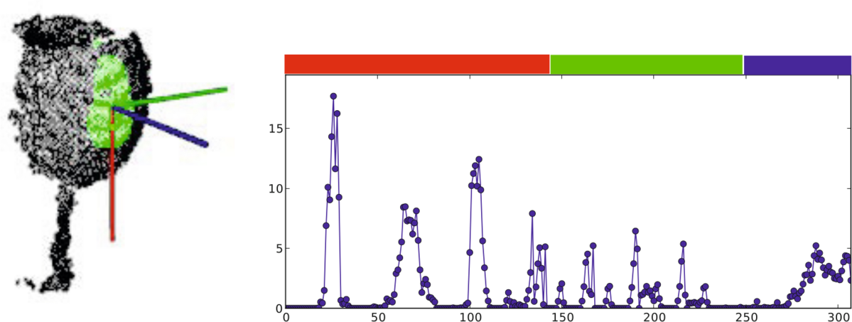
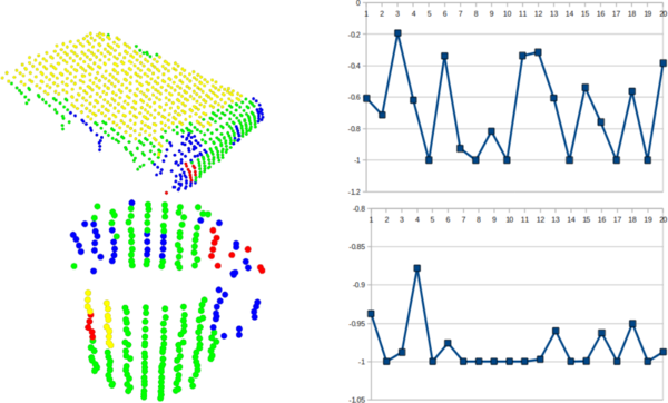
1.7 SI(Spin image)

Spin images computed for 3 points of a model

• SI는 1997년부터 사용된 가장 오래된 기술자이다. The Spin Image (SI) is the oldest descriptor we are going to see here. It has been around since 1997, but it still sees some use for certain applications.

• 원래는 폴리곤에서 사용하기 위해 설계 되었지만 최근에는 포인트클라우드에도 적용되었다. It was originally designed to describe surfaces made by vertices, edges and polygons, but it has been since adapted for point clouds.

• 다른 기술자들과 달리 결과물이 이미와 같은 형태이다. 따라서 기존 여러 방법으로 비교가 가능하다. The descriptor is unlike all others in that the output resembles an image that can be compared with another with the usual means.

• The support structure used is a cylinder, centered at the point, with a given radius and height, and aligned with the normal.

• This cylinder is divided radially and vertically into volumes.

• For each one, the number of neighbors lying inside is added up, eventually producing a descriptor.

• 성능향상을 위해 가중치와 보간법이 이용된다. Weighting and interpolation are used to improve the result.

• 최종 기술자는 그레이스케일 이미지 이다. 어두울수록 밀집도가 큼을 나타낸다. The final descriptor can be seen as a grayscale image where dark areas correspond to volumes with higher point density.

1.8 RIFT(Rotation-Invariant Feature Transform)

2D SIFT 컨셉 활용 , 색상 정보 필요

RIFT feature values at 3 different locations in the descriptor

• 유일하게 intensity정보를 필요로 하는 기술자 It is the only descriptor seen here that requires intensity information in order to compute it
  • intensitycan be obtained from the RGB color values
  • This means, of course, that you will not be able to use RIFT with standard XYZ clouds, you also need the texture.

동작 절차

1. In the first step, a circular patch (with the given radius) is fitted on the surface the point lies on.

   • This patch is divided into concentric rings, according to the chosen distance bin size.

2. Then, an histogram is populated with all the point's neighbors lying inside a sphere centered at that point and with the mentioned radius.

3. The distance and the orientation of the intensity gradient at each point are considered.

4. To make it rotation invariant, the angle between the gradient orientation and the vector pointing outward from the center of the patch is measured.

1.9 NARF(Normal Aligned Radial Feature)

포인트클라우드용 아님, Range Image 사용

• The only descriptor here that does not take a point cloud as input. Instead, it works with range images.

• A range image is a common RGB image in which the distance to the point that corresponds to a certain pixel is encoded as a color value in the visible light spectrum: the points that are closer to the camera would be violet, while the points near the maximum sensor range would be red.

• NARF also requires us to find suitable keypoints to compute the descriptor for.

• NARF keypoints are located near an object's corners, and this also requires to find the borders (transitions from foreground to background), which are trivial to find with a range image.

1.10 RoPS(Rotational Projection Statistics)

• Triangle mesh를 이용하는 기술자로 사전에 Mesh생성 작업이 필요 하다. RoPS feature is a bit different from the other descriptors because it works with a triangle mesh, so a previous triangulation step is needed for generating this mesh from the cloud.

  • 나머지 컨셉은 비슷하다. Apart from that, most concepts are similar.

• In order to compute RoPS for a keypoint,

  • the local surface is cropped according to a support radius, so only points and triangles lying inside are taken into account.
  • Then, a local reference frame (LRF) is computed, giving the descriptor its rotational invariance.

• A coordinate system is created with the point as the origin, and the axes aligned with the LRF.

• Then, for every axis, several steps are performed.

  • First, the local surface is rotated around the current axis.
  • The angle is determined by one of the parameters, which sets the number of rotations.
  • For each one, statistical information about the distribution of the projected points is computed,
  • and concatenated to form the final descriptor.

2. Global descriptors

If global descriptors are being used, a Camera Roll Histogram (CRH) should be included in order to retrieve the full 6 DoF pose

전역 기술자는 물체의 기하학 정보를 가지고 있다. Global descriptors encode object geometry.

전역 기술자는 개별 포인트들을 계산하는 대신 물체를 나타내는 모든 클러스터를 계산한다. They are not computed for individual points, but for a whole cluster that represents an object.

• 이때문에 후보군 추출을 위한 전처리(=세그멘테이션)이 필요 하다. Because of this, a preprocessing step (segmentation) is required, in order to retrieve possible candidates.

전역 기술자는 물체 인식이나 분류, 기하학적 분석(물체 타입, 모양), 자세 추정 등에 활용된다. Global descriptors are used for object recognition and classification, geometric analysis (object type, shape...), and pose estimation.

많은 지역 기술자를은 전역 기술자처럼 사용 할수도 있다. You should also know that many local descriptors can also be used as global ones.

• This can be done with descriptors that use a radius to search for neighbors (as PFH does).
• The trick is to compute it for one single point in the object cluster, and set the radius to the maximum possible distance between any two points (so all points in the cluster are considered as neighbors).

2.1 VFH(Viewpoint Feature Histogram)

The VFH is based on the FPFH.

Viewpoint component of the VFH	Extended FPFH component of the VFH

• FPFH가 물체의 포즈에 invariant하기 때문에 viewpoint 정보를 추가 하여 기능을 확장 하였다. Because the FPFH is invariant to the object's pose, the authors decided to expand it by including information about the viewpoint.

• Also, the FPFH is estimated once for the whole cluster, not for every point.

• 구성 The VFH is made up by two parts:

  • a viewpoint direction component, and
  • an extended FPFH component.

A. viewpoint direction component

• To compute the first one,
  • the object's centroid is found, which is the point that results from averaging the X, Y and Z coordinates of all points.
  • Then, the vector between the viewpoint (the position of the sensor) and this centroid is computed, and normalized.
  • The vector is translated to each point when computing the angle because it makes the descriptor scale invariant.

B. extended FPFH component

• The second component is computed like the FPFH (that results in 3 histograms for the 3 angular features, α, φ and θ), with some differences:
  • it is only computed for the centroid, using the computed viewpoint direction vector as its normal (as the point, obviously, does not have a normal),
  • and setting all the cluster's points as neighbors.

The resulting 4 histograms are concatenated to build the final VFH descriptor.

• 1 for the viewpoint component
• 3 for the extended FPFH component

By default, the bins are normalized using the total number of points in the cluster.

• This makes the VFH descriptor invariant to scale.

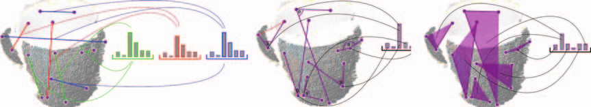
2.2 CVFH(Clustered Viewpoint Feature Histogram)

VFH 개선 버젼

• VFH는 가려짐등 센서의 영향에 간겅하지 못하다. The original VFH descriptor is not robust to occlusion or other sensor artifacts, or measurement errors.

  • If the object cluster is missing many points, the resulting computed centroid will differ from the original, altering the final descriptor, and preventing a positive match from being found.

• 아이디어는 간단하다. 전체 클러스터에 대해 single VFH을 계산 하는 대신 The idea is very simple: instead of computing a single VFH histogram for the whole cluster,

• 개선 방식 the object is

  • first divided in stable, smooth regions using region-growing segmentation, that enforces several constraints in the distances and differences of normals of the points belonging to every region.
  • Then, a VFH is computed for every region.

• 효과 : 최소 하나의 Region이 측정 가능하다면 물체를 찾을 수 있다. Thanks to this, an object can be found in a scene, as long as at least one of its regions is fully visible.

• 추가적으로 Additionally, a Shape Distribution Component (SDC) is also computed and included.

  • It encodes information about the distribution of the points arond the region's centroid, measuring the distances.
  • The SDC allows to differentiate objects with similar characteristics (size and normal distribution), like two planar surfaces from each other.

• histogram normalization절차 제거 The authors proposed to discard the histogram normalization step that is performed in VFH.

  • This has the effect of making the descriptor dependant of scale, so an object of a certain size would not match a bigger or smaller copy of itself.
  • It also makes CVFH more robust to occlusion.

• CVFH is invariant to the camera roll angle, like most global descriptors.

  • This is so because rotations about that camera axis do not change the observable geometry that descriptors are computed from, limiting the pose estimation to 5 DoF.
  • The use of a Camera Roll Histogram (CRH) has been proposed to overcome this.

2.3 OUR-CVFH (Oriented, Unique and Repeatable CVFH)

CVFH 개선버젼

SGURF frame and resulting histogram of a region

-강건성 확보를 위해 unique reference frame를 추가적으로 계산

• OUR-CVFH relies on the use of Semi-Global Unique Reference Frames (SGURFs),

  • which are repeatable coordinate systems computed for each region.

• SGURF적용 효과

  • Not only they remove the invariance to camera roll and allow to extract the 6DoF pose directly without additional steps,
  • but they also improve the spatial descriptiveness.

• The first part of the computation is akin to CVFH, but after segmentation, the points in each region are filtered once more according to the difference between their normals and the region's average normal.

  • This results in better shaped regions, improving the estimation of the Reference Frames (RFs).

• After this, the SGURF is computed for each region.

  • Disambiguation is performed to decide the sign of the axes, according to the points' distribution.
  • If this is not enough and the sign remains ambiguous, multiple RFs will need to be created to account for it.

• Finally, the OUR-CVFH descriptor is computed.

The original Shape Distribution Component (SDC) is discarded, and the surface is now described according to the RFs.

2.4 ESF(Ensemble of Shape Functions)

• ESF is a combination of 3 different shape functions(D2, D3, A3) that describe certain properties of the cloud's points:
  • distances,
  • angles
  • area.

• Normal정보를 필요로 하지 않는다. This descriptor is very unique because it does not require normal information.

• 별도의 전처리 작업을 필요로 하지 않지만, 노이즈와 incomplete surfaces에 대하여 강건성을 가진다. Actually, it does not need any preprocessing, as it is robust to noise and incomplete surfaces.

• The algorithm uses a voxel grid as an approximation of the real surface.

• 매 반복시 마다 3개의 점으로 랜덤하게 선별한다. It iterates through all the points in the cloud: for every iteration, 3 random points are chosen.

For these points, the shape functions are computed:

D2: 거리 계산 함수 this function computes the distances between point pairs (3 overall).

• Then, for every pair, it checks if the line that connects both points lies entirely inside the surface, entirely outside (crossing free space), or both.
• Depending on this, the distance value will be binned to one of three possible histograms: IN, OUT or MIXED.

D2 ratio: an additional histogram for the ratio between parts of the line inside the surface, and parts outside.

• This value will be 0 if the line is completely outside, 1 if completely inside, and some value in between if mixed.

D3: 세점으로 형성된 삼각형 면적의 square roo계산 this computes the square root of the area of the triangle formed by the 3 points.

• Like D2, the result is also classified as IN, OUT or MIXED, each with its own histogram.

A3: 각도계산 함수 this function computes the angle formed by the points.

• Then, the value is binned depending on how the line opposite to the angle is (once again, as IN, OUT or MIXED).

최종적으로 10개의 서브히스토그램 생성됨 After the loop is over, we are left with 10 subhistograms

• 9개 : IN, OUT and MIXED for D2, D3 and A3, and
• 1개 : an additional one for the ratio

Each one has 64 bins, so the size of the final ESF descriptor is 640.

2.5 G-FPFH (Global Fast Point Feature Histogram)

FPFH descriptor 전역 기술자로 확장

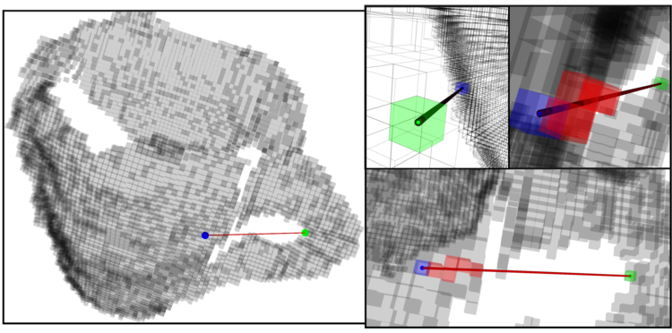Classification of objects made with FPFH and CRF	Computing the GFPFH with a voxel grid

목적 : 네비게이션에 도움을 주기 위하여 설계 됨 GFPFH was designed for the task of helping a robot navigate its environment, having some context of the objects around it.

[동작 과정]

1. 표면 분류(categorization) The first step before being able to compute the descriptor is surface categorization.

   • A set of logical primitives (the classes, or categories) is created, which depends on the type of objects we expect the robot to find on the scene.
   • For example, if we know there will be a coffee mug, we create three: one for the handle, and the other two for the outer and inner faces.

2. FPFH 기술자 계산 Then, FPFH descriptors are computed,

3. and everything is fed to a Conditional Random Field (CRF) algorithm.

   • The CRF will label each surface with one of the previous categories,
   • so we end up with a cloud where each point has been classified depending of the type of object (or object's region) it belongs to.

오늘날에 GFPFH 기술자는 분류 결과값을 가지고 계산 된다. Now, the GFPFH descriptor can be computed with the result of the classification step.

It will encode what the object is made of, so the robot can easily recognize it.

1. First, an octree is created, dividing the object in voxel leaves.

   • For every leaf, a set of probabilities is created, one for each class.
   • Each one stores the probability of that leaf belonging to the class, and it is computed according to the number of points in that leaf that have been labelled as that class, and the total number of points.

2. Then, for every pair of leaves in the octree, a line is casted, connecting them.

   • Every leaf in its path is checked for occupancy, storing the result in an histogram.
   • If the leaf is empty (free space), a value of 0 is saved.
   • Otherwise, the leaf probabilities are used.

2.6 G-RSD

The global version of the Radius-based Surface Descriptor works in a similar fashion to GFPFH.

Classification of objects for GRSD and resulting histogram

• A voxelization and a surface categorization step are performed beforehand, labelling all surface patches according to the geometric category (plane, cylinder, edge, rim, sphere), using RSD.

• Then, the whole cluster is classified into one of these categories, and the GRSD descriptor is computed from this.

1. Height Features

Descriptors

Toword3d2011alex

• Holistic descriptors

• Segment Descriptors

1. 객체 인식

   http://daddynkidsmakers.blogspot.com/2015/07/3.html

객체를 인식한다는 것은, 객체의 형상, 위치, 크기, 치수 및 속성값 등을 추출한다는 것이다. 세그먼테이션을 하였다면, 각 세그먼트마다, 이 속성값들을 추출하기 위해, 다양한 전략을 적용한다.

1) Hough Transformation 허프변환을 통해, 기본 형상의 단면에 대해 가장 잘 부합하는 치수를 찾는다. 허프변환은 2차원 비전에도 활용된 방식으로, 정규분포를 가정하고, 모델 치수의 평균값을 계산한다.

2) PFH Matching 인식하고자 하는 모델의 특징점 히스토그램을 미리 저장해 놓고, 입력되는 PCD에 대해, 이 값과 비교한다. 이는 2차원 비전에서 히스토그램 매칭과 같은 개념이다.

3) RANSAC 모델을 수학적으로 미리 정의해 놓는다. 그리고, 주어진 PCD의 샘플점을 획득해, 수학적 모델을 만들고, 이 모델과 PCD가 얼마정도 부합하지지 inlier 포인트 갯수를 계산한다. 이를 통해, 모델과 유사도를 계산해, 유사도가 미리 정의한 Tolerance 값을 넘으면, 그 모델의 수치가 PCD와 일치한 것으로 가정한다.

4) Curve fitting 커브 피팅은 주어진 PCD에 가장 일치하는 수학 모델의 계수값을 계산하는 방식이다. 예를 들어, 다음과 같은 모델 수식이 있다고 하면,

P(t) = ax + by + c

여기서, 주어진 포인트 P={x, y, z} 의 군 PCD에 대해, 이 모델 수식과 가장 잘 부합하는 a, b, c값을 찾는다. 이는 복잡한 수치해석이 필요하다.

5) ICP (Interactive Iterative Closest Point) 두개의 포인트 클라우드 PCD1, PCD2가 있을 경우, 각 PCD의 특징점 집합을 구해, 서로 위치가 같도록 (서로간의 거리가 가깝도록), 좌표 변환 행렬을 계산해 각 PCD에 적용한다. 그리고, 이 과정을 계산된 거리 편차가 Tolerance이하 일때까지 반복적으로 실행한다.

3.3 Features (7개)

Our feature vector per cluster consists of 8 different features introduced in the literature,

• where f1 and f2 are presented by Premebida et al. [17] and describe the number of points included in a cluster and the minimum distance of the cluster to the sensor.
• Navarro-Serment et al. [15] apply a Principal Component Analysis (PCA) to the clusters, which represents f3 to f7.

Those features are the 3D covariance matrix of a cluster, the normalized moment of inertia tensor, the 2D covariance matrix in different zones (cf. [15]), the normalized 2D histogram for the main plane and the normalized 2D histogram for the secondary plane.

In another approach, Kidono et al. [11] introduce two additional features.

• The first one, the slice feature of a cluster, forms our last feature f8 and aims to differentiate pedestrians from false positives in the shape of trees or poles.
  • A cluster is partitioned into slices along the z-axis and for each slice the first and second largest eigenvalue is calculated.
  • As the descriptive power of the slice feature decreases over longer distances, only a rough estimate remains in long distances.
• The other feature introduced by Kidono et al. considers the distribution of the reflection intensities in the cluster. -Since our LRF is not calibrated wrt. the intensities, this feature could not be integrated.

Confidence-Based Pedestrian Tracking in Unstructured Environments Using 3D Laser Distance Measurements

Point Cloud Processing: Estimating Normal Vectors and Curvature Indicators using Eigenvectors: ppt 17slide